Slump detector Using Statistics To Predict A Player's True Colors
Author: Andrew Scheiner
Slump Detector: Using Statistics to Predict a Player’s True Colors
This article will introduce a statistical method that can be used to analyze player performance over time. The sequential probability ratio test, or SPRT, is a statistical-based decision maker which can tell us a player’s true, or expected, performance over any number of sequential events. I will explain how SPRT can be used in a baseball context, specifically how a statistic like a player’s true batting average can be found by re-evaluating metrics after every single at-bat. This test can be extremely helpful for a variety of sports contexts. To name a few, we can use SPRT for detecting slumps versus expected improvement, which players to invest in for fantasy baseball, the best time to call a player up from the minors, and many more.
Deciding a Player’s True Hitting Ability
Let’s say you are the general manager of a baseball team. You want to determine if it is worth it to trade for a superstar baseball player who is slumping in the middle of the season. In this scenario, it is June, so we have a sample size of approximately 200 at-bats, and the player has a .230 batting average. This player historically has a career .270 average, but this season, they do not seem like the same hitter. SPRT allows us to take each at-bat, one at a time, and determine if the player’s true batting average is closer to say, a .200 hitter, or a .275 hitter. This is the difference between your league average hitter and a star. SPRT does not need a large sample size to make decisions, and we can even generate a line graph to see how the player’s true batting average similarity changes over time and different series of outcomes. By a series of outcomes, I am referring to hot streaks and cold streaks (the latter are slumps).
SPRT - a Simple Explanation
Requirements:
- Sequence of binary results (ex: Hit = 1, Out = 0)
- Lower threshold / null hypothesis (ex: Batting average
<= 0.200) - Upper threshold / alternative hypothesis (ex: Batting average
>= 0.275) - Probability of a false alarm (our
alphavalue) - Probability of a missed opportunity (our
betavalue)
Process:
- We use alpha and beta to create the odds thresholds for accepting each of our hypotheses.
- Convert each odds threshold to a
logvalue so we can compare with the log-likelihood ratio.- Log-likelihood ratio, aka LLR, is essentially a running total that tells us which hypothesis we should accept based on our thresholds.
- Compute the increments for LLR. How much will LLR change if (for example) the batter gets a hit or gets an out?
- Increment LLR based on each event sequentially.
- Check if we have a decision that we can make using SPRT. This is called our “check to stop”.
- In our context: if LLR is above our upper threshold, accept that the batter is a 0.275 hitter.
- If LLR is below our lower threshold, accept that the batter is a league-average hitter.
- We can check to stop after each result is processed, or we can wait for all results to be processed before checking.
SPRT Example
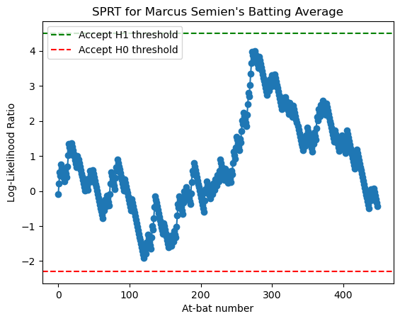
Let’s say we are the general manager of the Texas Rangers and we need to figure out whether Marcus Semien (their starting second baseman) should be traded because he is only a league-average hitter (0.200 batting average) or if we should keep him around because he is a star (0.275). We will say our acceptable chance for a false alarm is 1% and a missed opportunity is 10%. Using the 2025 season, here is Semien’s SPRT result for batting average:
- Our upper threshold is 4.5
- Our lower threshold is -2.3
- Every time Semien gets a hit, LLR increases by 0.32
- Every time Semien gets a hit, LLR decreases by 0.1
Here is the running total of LLR after Semien’s first ten at-bats of the season
- LLR after at-bat 1: -0.10
- LLR after at-bat 2: 0.22
- LLR after at-bat 3: 0.54
- LLR after at-bat 4: 0.44
- LLR after at-bat 5: 0.76
- LLR after at-bat 6: 0.66
- LLR after at-bat 7: 0.56
- LLR after at-bat 8: 0.46
- LLR after at-bat 9: 0.36
- LLR after at-bat 10: 0.27
If we were mid-season and needed to make a decision, here are some significant LLR values:
- LLR after at-bat 121: -1.91
- LLR after at-bat 277: 4.00
- LLR after at-bat 449: -0.43 (final at-bat)
At at-bat 121, we are almost at a confident decision to accept that Marcus Semien is a league-average hitter. This is because LLR at at-bat 121 is -1.91, which is almost less than -2. At at-bat 277, Semien’s LLR is 4, which is almost above our upper threshold of 4.5. So near the trade deadline, we would almost be able to make a confident decision that Semien is a star, so we would be inclined to not trade him. After Semien’s final at-bat, his LLR is -0.43. Since this is in-between our thresholds, we would need more results to make a decision. But since it was his final at-bat, we are unfortunately in between potential decisions. What’s fascinating about SPRT is how we can make decisions throughout the season based on sequential evidence.
Why Choose SPRT?
Sports are full of yes-or-no outcomes — hits or outs, wins or losses, success or failure. SPRT is built to handle those kinds of results. It looks at the data after every play or event, so you don’t have to wait for a huge sample before making a choice. Whether it’s calling up a minor leaguer, deciding on bullpen roles, testing defensive shifts, or trying new lineups, SPRT gives you a way to turn small bits of data into real decisions. In a world where teams want fast and smart answers, SPRT is a simple tool that helps make complex calls easier.
If you are interested in learning more about SPRT, its calculations, and the mathematical context behind the test using my baseball scenario, please see my section below for a “behind the scenes”.
SPRT - Behind the Scenes
SPRT is a hypothesis test, where we can make three decisions:
- Accept our null hypothesis (H0)
- Accept our alternative hypothesis (HA)
- Fail to conclude (1) or (2) - must continue sampling
A log-likelihood ratio (LLR) is then created to compute the ratio of probabilities under H0 vs. H1. This is a running total of results.
Typically,
H0: true value <= XHA: true value >= Y
where X and Y are two numeric values and Y > X.
We then create two thresholds using the following:
- Upper threshold (U) =
(1 - B) / a - Lower threshold (L) =
B / (1 - a)
where
a= Type 1 error, the probability of rejecting H0 when it is trueB= Type 2 error, the probability of failing to reject H0 when H1 is true
Each threshold is then converted to a log value.
For our usage of SPRT, we calculate LLR as we go. SPRT works with binary events. Thus, we must calculate an increment to LLR for both event = 1 and event = 0.
- Each
event = 1addsln(Y / X) - Each
event = 0subtractsln((1-Y)/(1-X))
from LLR.
After each event is counted while running SPRT, check the following conditions:
If LLR >= U: Accept H1Else if LLR <= L: Accept H0Else: Continue sampling
These conditions can be checked either (a) after each event is counted or (b) after all events have been counted.